
Today’s post ventures into unfamiliar territory for many of us, the pedagogy of equations and statistics. It is part of a series summarizing an economic article in HHTM’s Journal section entitled Supply and Demand for Audiologists.
If you think we’re down in the weeds again, where Econ 202 posts usually end up, you aren’t wrong. But there is method in the madness so please read on.
Besides, it’s the 4th of July so we don’t expect many readers of posts this week. Tune in next week when we pick up the summary of Supply and Demand of Audiologists again.
Central Tendencies and Parametric Stats — It’s a Start
Most audiologists take a basic course in statistics or research methods at some point in college, or as part of their graduate training. How else to read research in our own journals and understand how to interpret results described in terms of means, medians, variance, confidence levels, significance levels, risk levels, etc? How else to implement best practices in clinical settings, with a working understanding that what is best for 95 patients through the door may not be what is best for another 5?
But clinicians know that a single variable and measures of central tendency do not a patient, or a successful outcome, make. Anyone who has worked for even a short time with those who report hearing difficulties knows that the audiogram is a starting point at best and a red herring at worst when it comes to hearing aid fittings. Clinicians sense that some, maybe many, variables in the equation for successful treatment outcomes have yet to be nailed down, much less measured.
The Story Isn’t Complete and It’s Not Simple
A number of studies throughout the years have taken statistical stabs at identifying the formulary for successful hearing aid fitting outcomes, using survey responses (e.g., MarkeTrak), retrospective and occasionally prospective studies. Most recently, our field has taken up large data sets made available from ongoing epidemiological studies (e.g., NHANES) to grab more variables and see if they contribute to the formula for fitting success.
It is hard to keep so many variables in one’s head, much less give each its due, even when the equations signal their relative importance or lack thereof. Perhaps this is why there is a strong tendency to single out a heuristic1 variable (e.g., price) as the main mover and shaker even though it not justified by the analyses.
This natural, but erroneous, tendency to pare down and explain all in “simple” terms is manifest even among those who navigate comfortably in the statistical maze and perform some of the epidemiological work. How else to explain why the present social policy discussions identify cost and access as the clear and present villains which prevent all from wearing hearing aids, when even the most basic analyses make it equally clear that this thinking is over simplified at best and almost certainly wrong in most cases.
Could it be that many people do not prefer hearing aids at any cost point when they assess other choices for how to spend their time and money?
Using Models to Predict Outcomes
All of the above is a thought exercise bringing readers to the point of today’s post. In order to keep many potentially relevant variables in our heads, we need to step up our game and familiarize ourselves with a tool or two from basic econometrics, which Investopedia straight-forwardly defines as “…the application of statistical and mathematical theories … for the purpose of testing hypotheses and forecasting future trends.”
Count the Squares
Here’s a brief primer on one tool called OLS regression, where OLS = Ordinary Least Squares. The goal of OLS, like other regression methods, is to go beyond correlation and find causation by identifying determinants of outcomes.
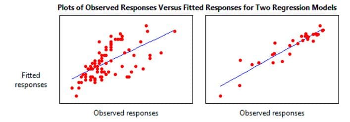
Figure 1. Examples of relative success of a linear model at “fitting” observed data. The smaller the variance of observed responses (the squares of standard deviations) from the line, the closer the fit. Hence the name, “least squares.”
Start with a single regressor linear model:
Y = ß0 + ß1X1 + ε
and consider how Y changes with every 1-unit change in X.
Algebraically, we know that this plots as a line which intersects the y axis at ß0 and has a slope of ß1. What OLS does is compare actual values of Y (e.g., our hearing aid outcomes for N subjects) to predicted values of Y, based on the line estimated by the equation.
The success of the OLS model hinges on how small the average squared differences (the variances) are between actual and predicted values – the smaller the variance, the better the predicted fit. That is measured by “R2”, the coefficient of determination (c.f. Figure 1).
The model breaks down as follows:
Dependent Variable Y: This is the effect, the outcome, we’re measuring. For instance, Y could be a scale of patient-reported hearing aid satisfaction from 1 to 10.
Constant/Intercept β0: Y depends on some constant which we don’t care much about that is β0 (it is what it is). For example, all those observations in the dataset may come from subjects who at least 60 years old, so the regression “starts” at 60.
Independent (Regressor) Variable X: What we do care about is what measureable variable (e.g., patient age) could “cause” our outcome to change. That potential influencer is X1, where the subscript denotes each subject in the dataset, from 1 to n.
Regression Coefficient ß1: Maybe age does predict hearing aid satisfaction, but if it does, then by how much and in what direction (i.e., does satisfaction grow or diminish with age)? ß1 multiples the regressor variable and therefore determines its magnitude and sign. When it’s 0, we know that X (age) has no effect on Y (hearing aid satisfaction) . The bigger ß1 is, the more our model “expects” that X affects Y. When ß1 is negative, the model predicts an inverse relationship between X and Y; when positive, we expect that Y grows as X grows.
Going back to the model and plugging in some made-up numbers, if
Y = 60 + (-0.5)X1 + ε
then we expect hearing aid satisfaction to decline a half-point on the 1 to 10 scale with every 1-year increase in age, all other things held constant.
Error term ε: It’s simplistic to expect age or any other single variable to explain 100% of hearing aid satisfaction. Which is why the model has ε . That “noise” variable is everything else that independently influences hearing aid satisfaction, essentially everything that our single-regressor variable model doesn’t explain.
With the simple model above, you can be sure that ε is going to be big and a lot of “other things” have to be held constant in order for age to “predict” hearing aid satisfaction.
More Independent Influencers, Less Noise, Better Prediction
Which is why it’s better to use a model with multiple regressors, so long as the regressors aren’t themselves related (e.g., age and blood pressure tend to vary together so they can’t serve as independent regressors in the same model). That would violate the assumption of collinearity, which is one of several assumptions required of the model (and not discussed here).
Eventually, the linear model looks like this:
Y = ß0 + ß1X1 + β2X2 + β3X3 … βjXj + ε
Where there are 1 through j “vector” variables and the expected contribution of each variable on, for instance, hearing aid satisfaction (when the others are held constant) can be seen by the size of the respective correlation coefficients, β1…j.
Finally, within the model, we can apply statistical tests to test the research and null hypotheses (H1 and H0) by calculating the probability and stating a level of confidence that a given variable does or does not significantly affect hearing aid outcome. As for the overall model, R2 tells us what percent of the variance in hearing aid satisfaction is explained by the model.
A Tool Set We Can Use
Most audiologists are not going to run out and start modeling data, even if their math and stat skills allow for it. But, all audiologists will feel good about being able to look at a regression equation and understand what variables are influencing whatever outcome the model is trying to predict.
The take-home is that methods exist which allow us to test assumptions about what factors influence consumer decisions to purchase and use of hearing aids, choose a provider, etc. Price and access are likely determinants, but so are many other variables we can and should plug into our models.
Footnotes
1Heuristics in psychology refer to “mental shortcuts that usually involve focusing on one aspect of a complex problem and ignoring others.” Wikipedia
images from wikihow & minsitab