Before the Audiogram

Audiogram, AW’-dee-oh-gram”, (n). A record of the threshold of sensitivity of hearing measured at several different (usually discrete) frequencies{{1}}[[1]]Modified slightly from Delk, J.H. Comprehensive Dictionary of Audiology, P 35, 1973, The Hearing Aid Journal, Sioux City, IA[[1]].

Strange as it may seem to many currently measuring and recording hearing results, the audiogram did not always portray hearing sensitivity as logically as it does today. Historically, there was not a systematic organizational sequence to the audiogram’s development until about the time of the audiometer.

The concept of the audiogram did not exist when hearing first began to be assessed. It seems to have emerged later in a rambling way to graphically or numerically record results from the various specialties in hearing at the time – otology, physics, engineering, psychoacoustics, which all pre-date the discipline of audiology as it is known today. Recording results of measurements that reflected the condition of a person’s hearing seems to have been born out of the need for hearing scientists and otologists to observe, measure, and record hearing behavior{{2}}[[2]] Hedge, M. N. (1987). Observation and measurement. In Clinical research in communicative disorders (pp. 105–106) Boston: College-Hill Press[[2]].

Not surprisingly, the historical development of the audiogram as a tool for daily use arouses little enthusiasm among those measuring hearing. After all, it’s just a form! How exciting can the generation of a form be? Perhaps not exciting, but it follows and reflects the historical development of ear pathology as well as the methods by which the ear’s function came to be understood. As knowledge of the ear’s performance grew, there grew also a desire to systematically collect and compare results.

This post focuses on what might be called the pre-audiogram expression of hearing test results. A detailed explanation of the actual audiogram development can be found in an excellent article by Jerger{{3}}[[3]]Jerger, J. Why the audiogram is upside down, The Hearing Review, March 27, 2013[[3]].

Developments Leading to the Audiogram Chart

Auditory Chart
One of the first foundations of the audiogram may be the “Auditory Chart” designed by Arthur Hartmann in 1885 to record tuning fork results{{4}}[[4]] Feldman, H. (1970). A history of audiology; A comprehensive report and bibliography from the earliest beginnings to the present, Translations of the Beltone Institute for Hearing Research, No 22[[4]]. As illustrated in Figure 1, seven tuning forks of different frequencies were used to determine how long the listener could respond to the tone. This was performed for the right and left ears separately. The frequencies measured used the following tuning forks; C (64 Hz), c (128 Hz), c1 (256 Hz), c2 (512 Hz), c3 (1024 Hz), c4 (2048 Hz), and c5 (4096 Hz).

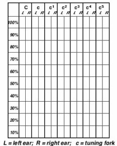
Figure 1. Hartmann’s “Auditory Chart,” conceived in 1885. This was used to report tuning fork responses from the left and right ears, using seven different tuning fork frequencies (C, c, c1, c2, c3, c4, and c5). This illustration has been enhanced from a recreation of Hartmann’s Auditory Chart by Vogel, et. al, 2007.

A meaningful example of Hartmann’s Auditory Chart for plotting is shown in Figure 2, which reduced the number of tuning forks to six, from seven{{5}}[[5]]Hartmann, A. Translated by J. H. Shorter, The graphic representation of the results obtained by testing the hearing with tuning-forks, On the Diseases of the Ear and their Treatment; 3rd edition, 1885. Deutsche Mediz. Wochenschrift, No. 15, 1885[[5]]. The scale was divided vertically into 100 equal parts, and the charts were arranged so that the upper half registered the air-conduction results, and the lower half those from bone conduction.

Tuning forks were chosen that had a vibratory duration from 30 to 60 seconds for the normal ear, and an average of numerous measurements was used to provide the reference number durations at the bottom of both portions of the graph. Duration times for bone conduction (lower part of graph) are less than for air conduction, which would be expected.

The proportion of time heard to normal durations, calculated in percentage, is of the time that the tuning fork is heard by the impaired ear, to the time determined as the average for the normal ear. (Example: upper graph, tuning fork A, right ear in red – signal is heard for 5 seconds, and for a “normal” hearing listener was averaged for this tuning fork to be 20 seconds; 5 seconds, divided by 20 seconds results in a “heard” percentage of 25%). Results are registered in colors on this graph (the original graph represented the ears by different black and white hash marks) representing the right and left ears in the spaces allotted for the several tuning forks.

At the time, the bone-conduction results were not registered in proportion to the normal standard Hartmann found for bone conduction, but instead he recorded these in relation to the average normal hearing by air conduction. This enabled Hartmann to make better and more direct comparisons between the air- and bone-conduction results. Recognition that bone-conduction vibratory duration is much shorter than for air-conduction was noted, and actually shown in this graph. From these plottings, Hartmann interpreted the resulting configurations into seven different hearing categories.

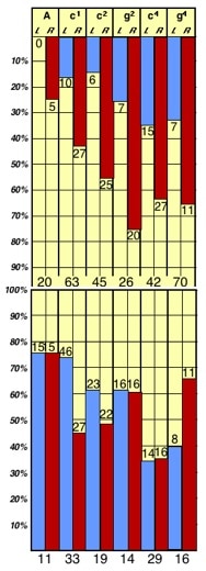
Figure 2. “Auditory Chart” by Hartmann (1885) reporting responses in duration in proportion (internal numbers) to “normalized” durations (bottom of each portion of the chart) for normal listeners. (Redrawn from original charts by Staab, 2014).

Hartmann calculated the duration of the normal ear by air-conduction, using selected tuning forks, to be 20, 63, 45 seconds, etc., as shown in the center of the graph. The pathological ear durations are recorded in figures representing the proportionate value for each of the tuning fork test frequencies and are shown in the upper graph. The lower end of the chart was used to record the vibratory durations for the normal ear by bone conduction (e.g., 11, 33, 19, etc.). Again, the numbers plotted represent their proportion to the normal hearing by air-conduction. Hartmann commented, “The diagrams thus obtained are so clear and characteristic that one can immediately tell what form of deafness we are dealing with without the necessity of any further explanations.”

The Auditory Chart of Hartmann provided duration numbers that could be compared between air- and bone-conduction tuning forks, providing some resemblance to current audiograms. However, the “norms” were questionable, and the chart provided no information about the hearing levels relative to hearing “sensitivity” other than the subjective “norms” Hartmann established for his set of selected tuning forks. Regardless, the graphics now began to resemble a chart with numbers representing values and “norms” for different frequencies for comparison purposes.

Acumetric Schema
Politzer, Gradenigo, and Delsaux (1904) proposed a method to document hearing sensitivity measurements and to provide a “standard” for terminology. This was still the age of tuning fork hearing measurements, which are reflected in the form (Figure 3). Their proposal was presented at the 7th International Congress of Otology in Bordeaux, France, but was not accepted until the 8th International Congress of Otology in Budapest, Hungary the following year. Not shown on the chart were their attempts to standardize nomenclature for “auditory area” and “auditory horizon.” However, their proposal was never universally accepted (Feldman, 1970).

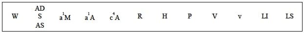
Figure 3. Acumetric Schema proposed by Politzer, et. al., in 1904 as a standard for reporting results of hearing measurements using tuning forks. Key: W = Weber test; AD = auris dextra (right ear); S = Schwabach test; AS = auris sinistra (left ear); a1M = duration of the auditory sensation with a fork placed on the mastoid; a1A = same for air conduction; c4A = same for a c4 fork and air conduction; R = Rinne test; H = horlogium (distance that a watch may be heard); P = results of Politzer’s acumeter; V = vox (distance to which conversational speech is understood); v = same for whispered voice; LI = limes inferior (lower frequency limit); LS = limes superior (upper frequency limit){{6}}[[6]] Vogel, D.A., McCarthy, P.A., Bratt, G. W., Brewer, C. The clinical audiogram: its history and current use, Communicative Disorders Review, Vol. 1, No 2, 2007, pp 81-94[[6]].

Still Missing – Quantitative Values Relative to Normal Hearing
Any reporting graph, to be meaningful, should have some quantitative measure relative to normal. Up to this point, evaluators selected intensity steps arbitrarily.

Max Wien’s Sensitivity Curve
In 1903, Max Wien presented a “Sensitivity Curve,” or audibility curve using a telephone receiver (Figure 4). Original on this chart was the sensitivity scale along the ordinate, relating these to the commonly used different frequency tuning forks. This showed fixed absolute intensity thresholds for frequencies between 50 and 12,000 Hz. The maximum sensitivity near 2200 Hz was 10⁸ times that at 50 Hz. Later work by Wegel (1922) at the Bell Telephone Laboratories (Figure 5) further mapped the auditory area, including the dynamic range (threshold of audibility and threshold of feeling), showing the absolute threshold to be well below 0.001 dyne cm^-2 at 220 Hz. So, although Wien’s results were in error, the results of the exercise were clear:
1. The upper and lower limits of audibility of pitch depend entirely on the intensities at which the measurements are made, and
2. The ear is a very sensitive device that rivals the eye.

Wien’s “Sensitivity Graph” appears to be the first graph showing the relationship between hearing thresholds (sensitivity) and frequency.

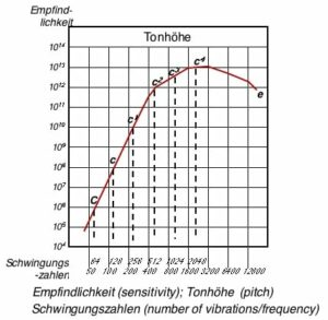
Figure 4. Sensitivity curve of Wien. This is reported to be the first graph to show the relationship between hearing sensitivity and frequency, presented in 1903.

However, it was not until 1922 that the boundaries of hearing sensitivity by frequency appeared when the frequency sensitivity of normal ears in dynes/cm2 was first represented on an intensity logarithmic scale as reported by Fletcher and Wegel (Figure 5) {{7}}[[7]]Fletcher, H., and Wegel, R. The frequency-sensitivity of normal ears, Proc. Natl Acad Sci USA. Jan 1922; 8(1): 5-6.2[[7]] .

The audible area of man was mapped further by Wegel (from Fletcher, 1970), as shown in Figure 6{{8}}[[8]]Fowler, E.P., Wegel, R.L., 1922.  Audiometric methods and the application.  Transactions of the 28th Annual Meeting of the American Laryngological, Rhinological and Otological Society, pp. 98-132[[8]].

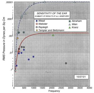
Figure 5. Frequency sensitivity of normal ears in dynes/cm2 as reported by Fletcher and Wegel, 1922 and represented on an intensity logarithmic scale. (This image has been enhanced from its original by Staab, 2014).

Even though substantial work had been performed in the preceding fifty years to determine the absolute minimum amount of sound that the human ear could perceive, the results varied widely. This problem was solved with the development of the vacuum tube, condenser microphone, and thermal receiver. By use of a specially constructed attenuator, the receiver current could be varied approximately three millionfold by moving a single dial switch. “By means of condenser transmitters and thermal receivers, this system was calibrated so that from the reading of the attenuator dial switch and the electric current entering it, the alternating pressure impressed upon the ear cavity could be determined in dynes per square centimeter” (Fletcher and Wegel, 1922). In making the measurement, the vacuum tube oscillator was set to a desired frequency. The attenuator was then moved until the sound from the receiver (at the ear) reached the various thresholds of audibility. The result is shown in Figure 6.

Figure 6. The frequency-intensity and pitch-loudness limits of the human ear, or what is called the audible area of man. (After Wegel, from Fletcher, 1923).

Actual Developments That Defined the Audiogram – Jerger Article
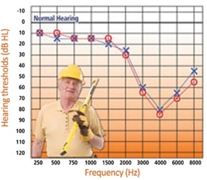
The graph in Figure 6 now has some characteristics that might be vaguely identified with today’s audiogram, specifically the frequency and intensity scales. However, the necessary auditory area, including detailed normal hearing sensitivity, frequency range, dynamic range of hearing, tolerance levels, etc. awaited the functional development of the audiometer.

In order to complete the final steps to the audiogram as we know it today, and to fill in other historical information omitted in this post, the reader is encouraged to read the excellent article written by Dr. James Jerger that explains the audiogram and how it came to be represented as it is (Jerger, 2013).